Performance

Where possible, all functions are written using numpy to make use of optimized routines and vectorization. Evaluating a single point typically takes less than 0.0001 seconds on a modern desktop system, regardless of function. This page shows some more detailed information about the performance, even though this library should not be a bottleneck in any programs.

The scripts for generating following performance overviews can be found in the docs/scripts folder of the repository. Presented running times were measured on a desktop PC with an Intel Core i7 5820k 6-core CPU, with Python 3.6.3 and Numpy 1.18.4.

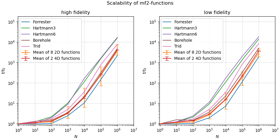
Performance Scaling

The image below shows how the runtime scales as N points are passed to the functions simultaneously as a matrix of size (N, ndim). Performance for the high- and low-fidelity formulations are shown separately to give a fair comparison: many low-fidelities are defined as computations on top of the high-fidelity definitions. As absolute performance will vary per system, the runtime is divided by the time needed for N=1 as a normalization. This is done independently for each function and fidelity level.

Up to N=1_000, the time required scales less than linearly thanks to efficient and vectorized numpy routines.

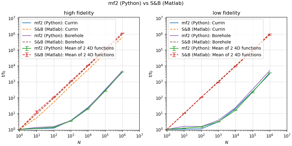
Performance Comparison

The following image shows how the scaling for the mf2 implementation of the Currin, Park91A, Park91B and Borehole functions compares to the Matlab implementations by Surjanovic and Bingham, which can only evaluate one point at a time, so do not use any vectorization. Measurements were performed using Matlab version R2020a (9.8.0.1323502).