Example Usage
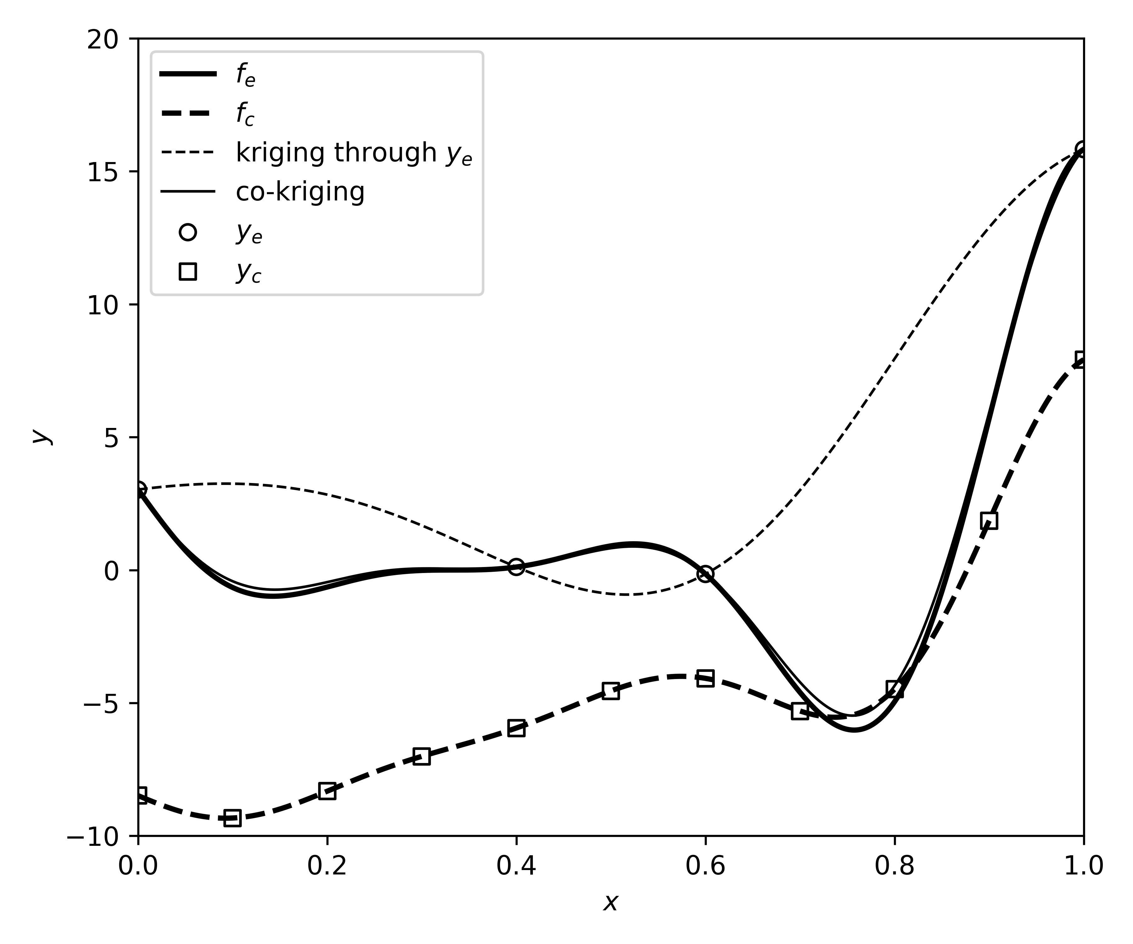
This example is a reproduction of Figure 1 from http://doi.org/10.1098/rspa.2007.1900 :
The original figure:

Code to reproduce the above figure as close as possible:
1 2 3 4 5 6 7 8 9 10 11 12 13 14 15 16 17 18 19 20 21 22 23 24 25 26 27 28 29 30 31 32 33 34 35 36 37 38 39 40 41 42 43 44 45 46 47 48 49 | # Typical imports: Matplotlib, numpy, sklearn and of course our mf2 package import matplotlib.pyplot as plt import mf2 import numpy as np from sklearn.gaussian_process import GaussianProcessRegressor as GPR from sklearn.gaussian_process import kernels # Setting up low_x = np.linspace(0, 1, 11).reshape(-1, 1) high_x = low_x[[0, 4, 6, 10]] diff_x = high_x low_y = mf2.forrester.low(low_x) high_y = mf2.forrester.high(high_x) scale = 1.87 # As reported in the paper diff_y = np.array([(mf2.forrester.high(x) - scale * mf2.forrester.low(x))[0] for x in diff_x]) # Training GP models kernel = kernels.ConstantKernel(constant_value=1.0) \ * kernels.RBF(length_scale=1.0, length_scale_bounds=(1e-1, 10.0)) gp_direct = GPR(kernel=kernel).fit(high_x, high_y) gp_low = GPR(kernel=kernel).fit(low_x, low_y) gp_diff = GPR(kernel=kernel).fit(diff_x, diff_y) # Using a simple function to combine the two models def co_y(x): return scale * gp_low.predict(x) + gp_diff.predict(x) # And finally recreating the plot plot_x = np.linspace(start=0, stop=1, num=501).reshape(-1, 1) plt.figure(figsize=(6, 5), dpi=600) plt.plot(plot_x, mf2.forrester.high(plot_x), linewidth=2, color='black', label='$f_e$') plt.plot(plot_x, mf2.forrester.low(plot_x), linewidth=2, color='black', linestyle='--', label='$f_c$') plt.scatter(high_x, high_y, marker='o', facecolors='none', color='black', label='$y_e$') plt.scatter(low_x, low_y, marker='s', facecolors='none', color='black', label='$y_c$') plt.plot(plot_x, gp_direct.predict(plot_x), linewidth=1, color='black', linestyle='--', label='kriging through $y_e$') plt.plot(plot_x, co_y(plot_x), linewidth=1, color='black', label='co-kriging') plt.xlim([0, 1]) plt.ylim([-10, 20]) plt.xlabel('$x$') plt.ylabel('$y$') plt.legend(loc=2) plt.tight_layout() plt.savefig('../_static/recreating-forrester-2007.png') plt.show() |
Reproduced figure: